3 Sampling Methods
3.1 Sample Size
3.1.1 Standard Error
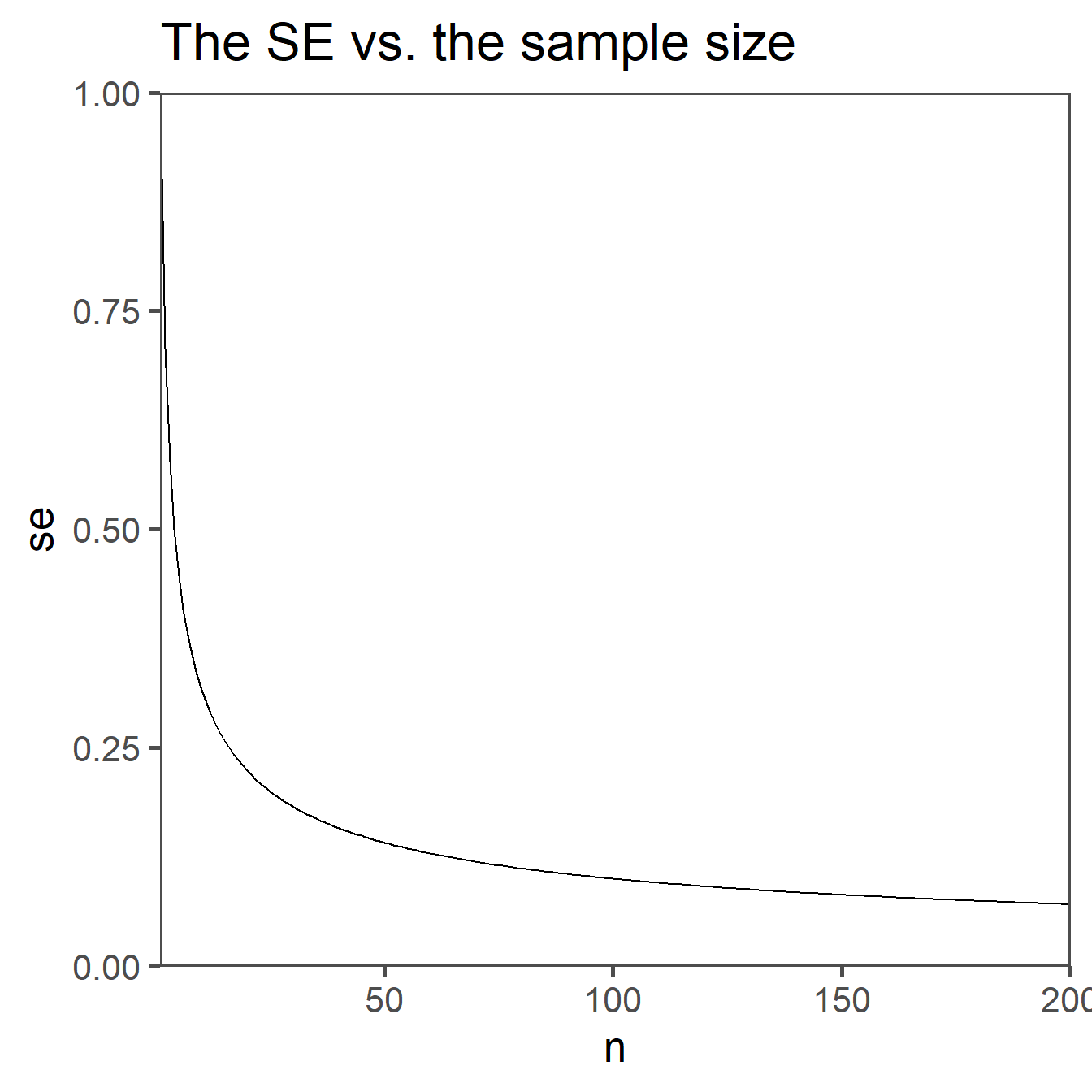
Standard Error (SE) is a statistical measure that quantifies the variation or uncertainty in sample statistics, particularly the mean (average). It is a valuable tool in inferential statistics and provides an estimate of how much the sample mean is expected to vary from the true population mean.
\[\begin{align} SE = \frac{sd}{\sqrt{n}} \end{align}\]
A smaller SE indicates that the sample mean is likely very close to the population mean, while a larger standard error suggests greater variability and less precision in estimating the population mean. SE is crucial when constructing confidence intervals and performing hypothesis tests, as it helps in assessing the reliability of sample statistics as estimates of population parameters.
Variance vs. Standard Deviation: The standard error formula is based on the standard deviation of the sample, not the variance. The standard deviation is the square root of the variance.
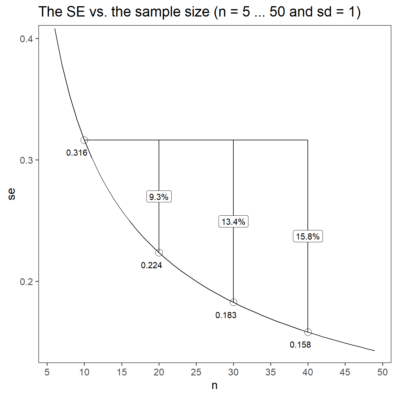
Scaling of Variability: The purpose of the standard error is to measure the variability or spread of sample means. The square root of the sample size reflects how that variability decreases as the sample size increases. When the sample size is larger, the sample mean is expected to be closer to the population mean, and the standard error becomes smaller to reflect this reduced variability.
Central Limit Theorem: The inclusion of \(\sqrt{n}\) in the standard error formula is closely tied to the Central Limit Theorem, which states that the distribution of sample means approaches a normal distribution as the sample size increases. \(\sqrt{n}\) helps in this context to ensure that the standard error appropriately reflects the distribution’s properties.
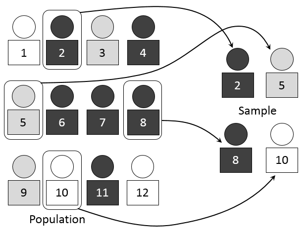
3.2 Random Sampling
- Definition: Selecting a sample from a population in a purely random manner, where every individual has an equal chance of being chosen.
- Advantages:
- Eliminates bias in selection.
- Results are often representative of the population.
- Disadvantages:
- Possibility of unequal representation of subgroups.
- Time-consuming and may not be practical for large populations.
3.3 Stratified Sampling
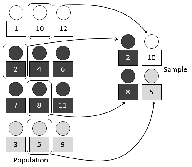
- Definition: Dividing the population into subgroups or strata based on certain characteristics and then randomly sampling from each stratum.
- Advantages:
- Ensures representation from all relevant subgroups.
- Increased precision in estimating population parameters.
- Disadvantages:
- Requires accurate classification of the population into strata.
- Complexity in implementation and analysis.
3.4 Systematic Sampling
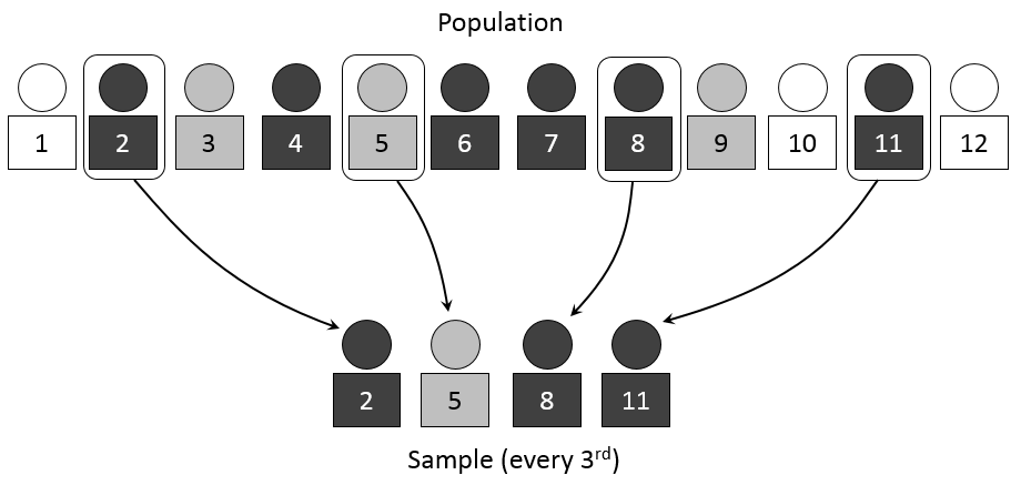
- Definition: Choosing every kth individual from a list after selecting a random starting point.
- Advantages:
- Simplicity in execution compared to random sampling.
- Suitable for large populations.
- Disadvantages:
- Susceptible to periodic patterns in the population.
- If the periodicity aligns with the sampling interval, it can introduce bias.
3.5 Cluster Sampling
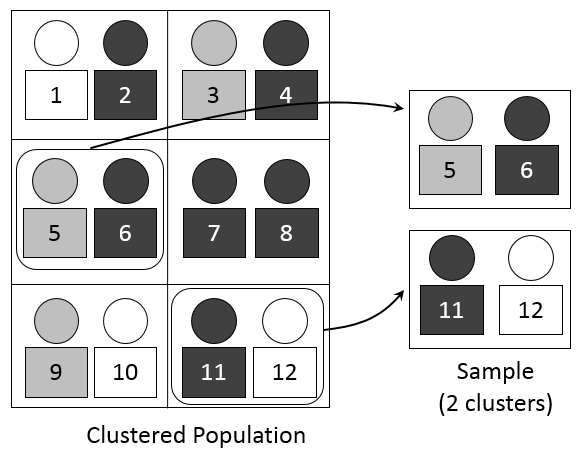
Definition: Dividing the population into clusters, randomly selecting some clusters, and then including all individuals from the chosen clusters in the sample.
Advantages:
- Cost-effective, especially for geographically dispersed populations.
- Reduces logistical challenges compared to other methods.
Disadvantages:
- Increased variability within clusters compared to other methods.
- Requires accurate information on cluster characteristics.
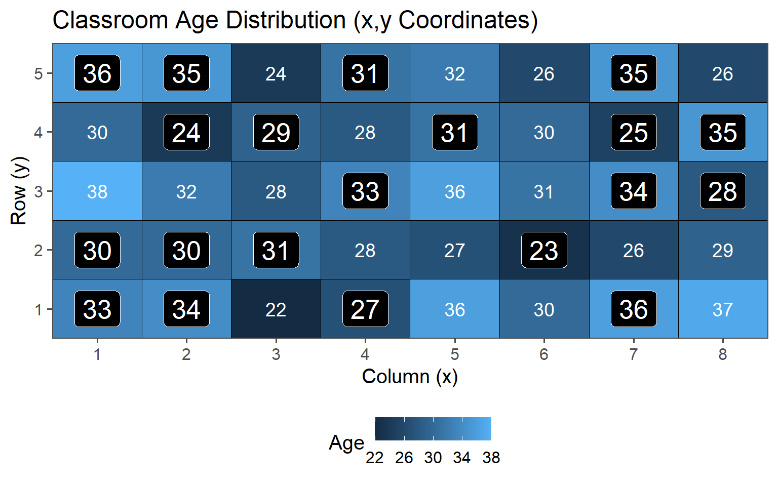
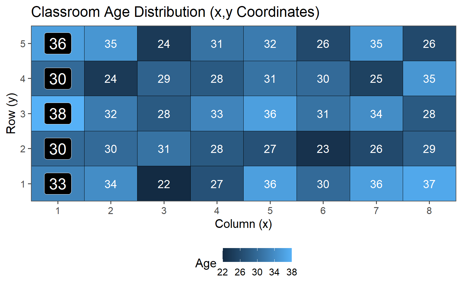
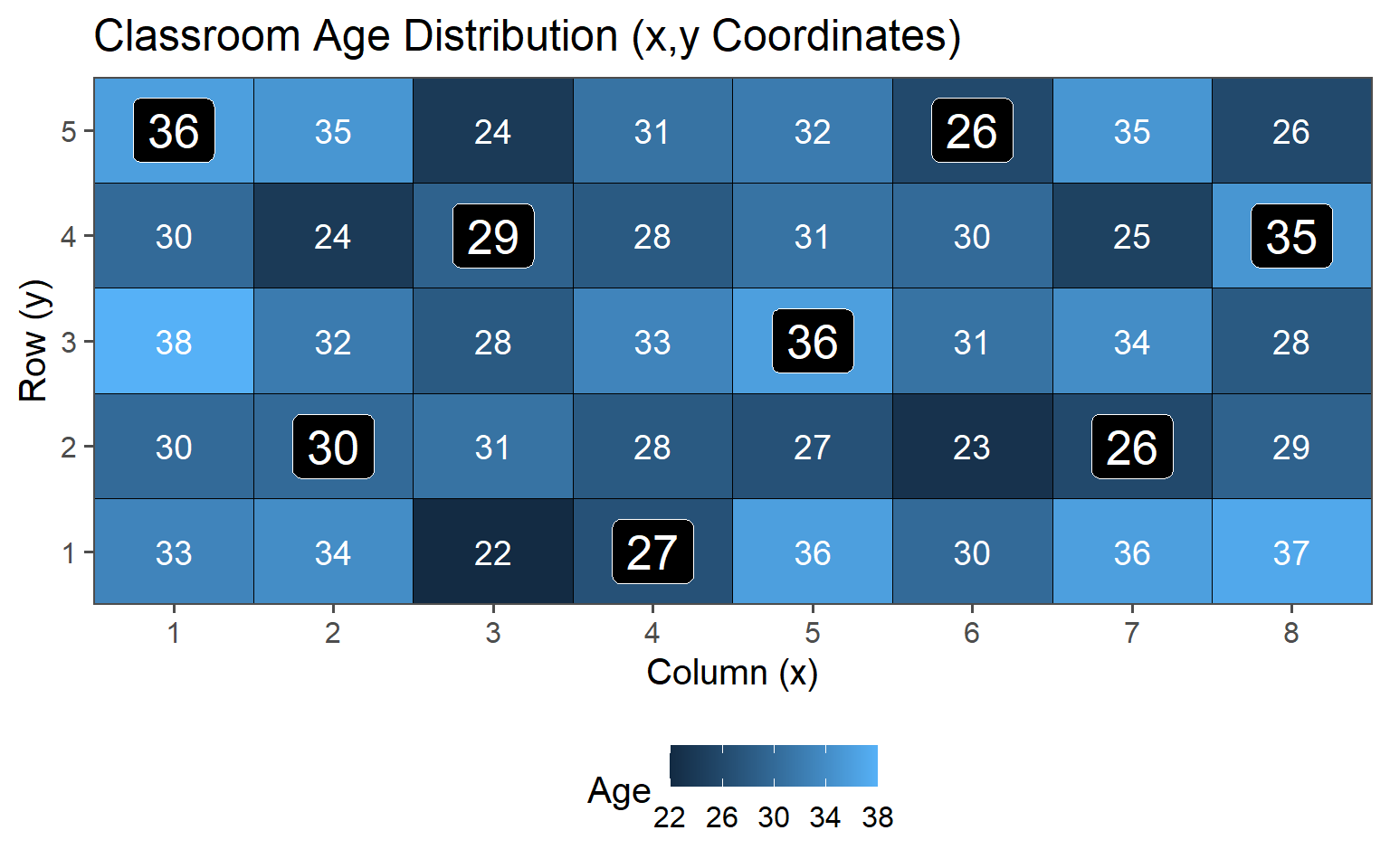
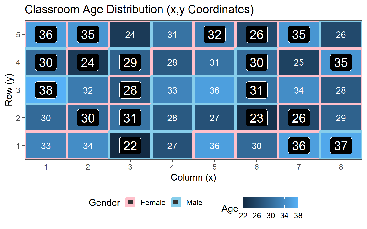
3.6 Example - Classroom Sampling
3.6.1 Descriptive Statistics (Population)
| Characteristic | N = 401 |
|---|---|
| Age | 30 (28, 34) |
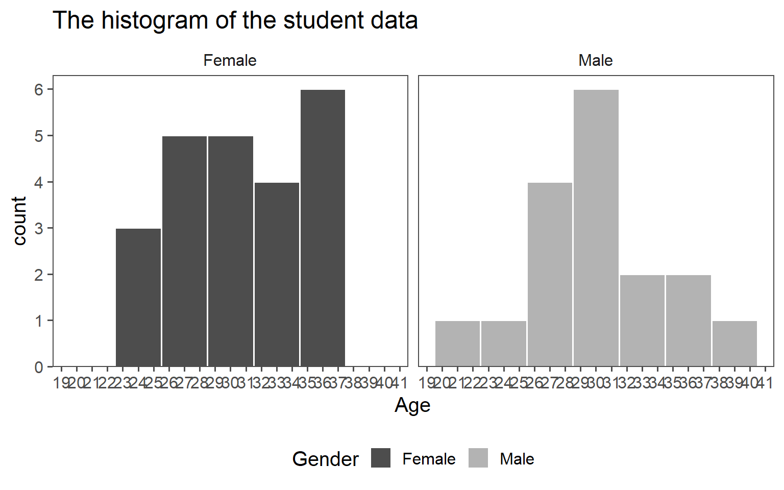
| Gender | |
| Female | 23 (58%) |
| Male | 17 (43%) |
| 1 Median (Q1, Q3); n (%) | |
3.6.1.1 Histogram
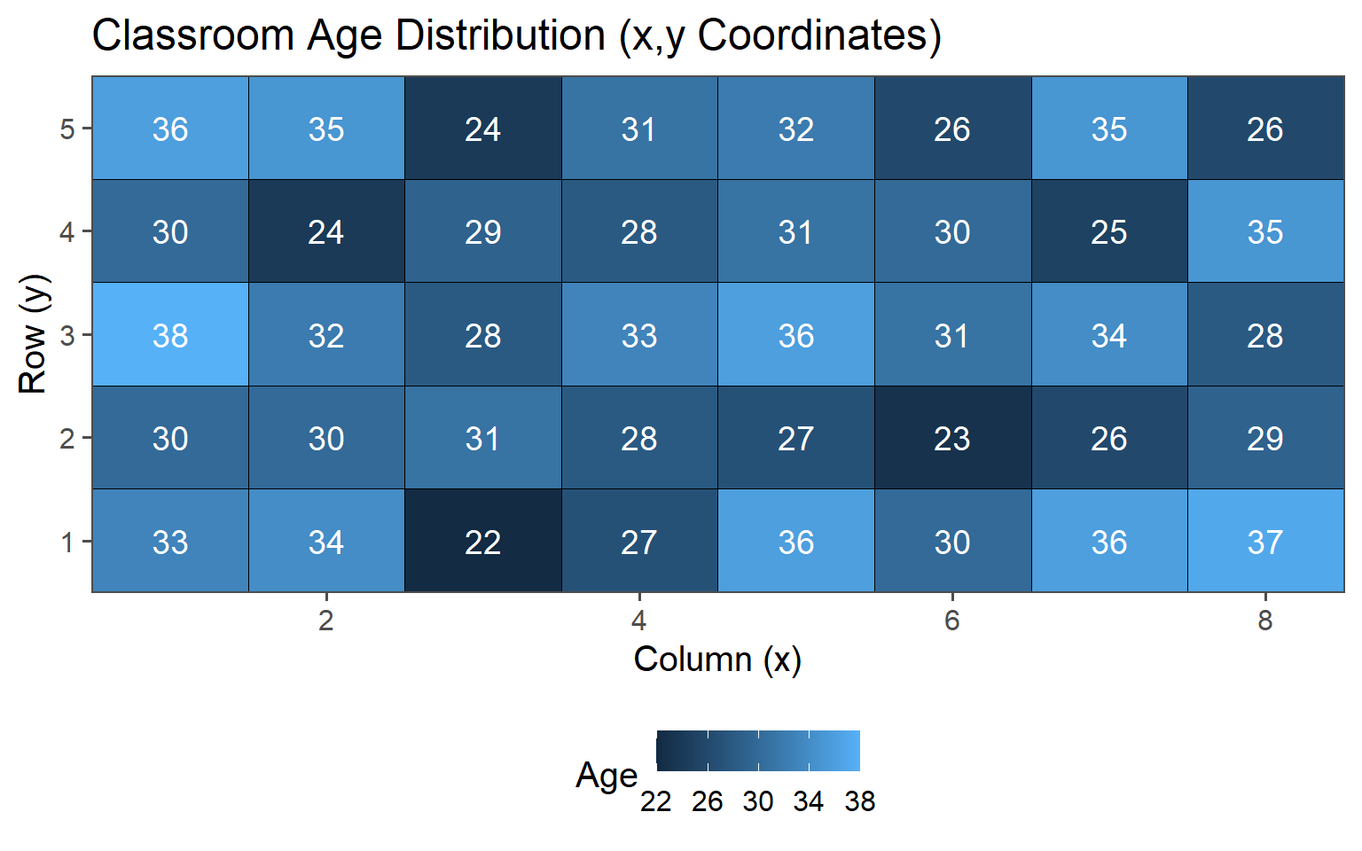
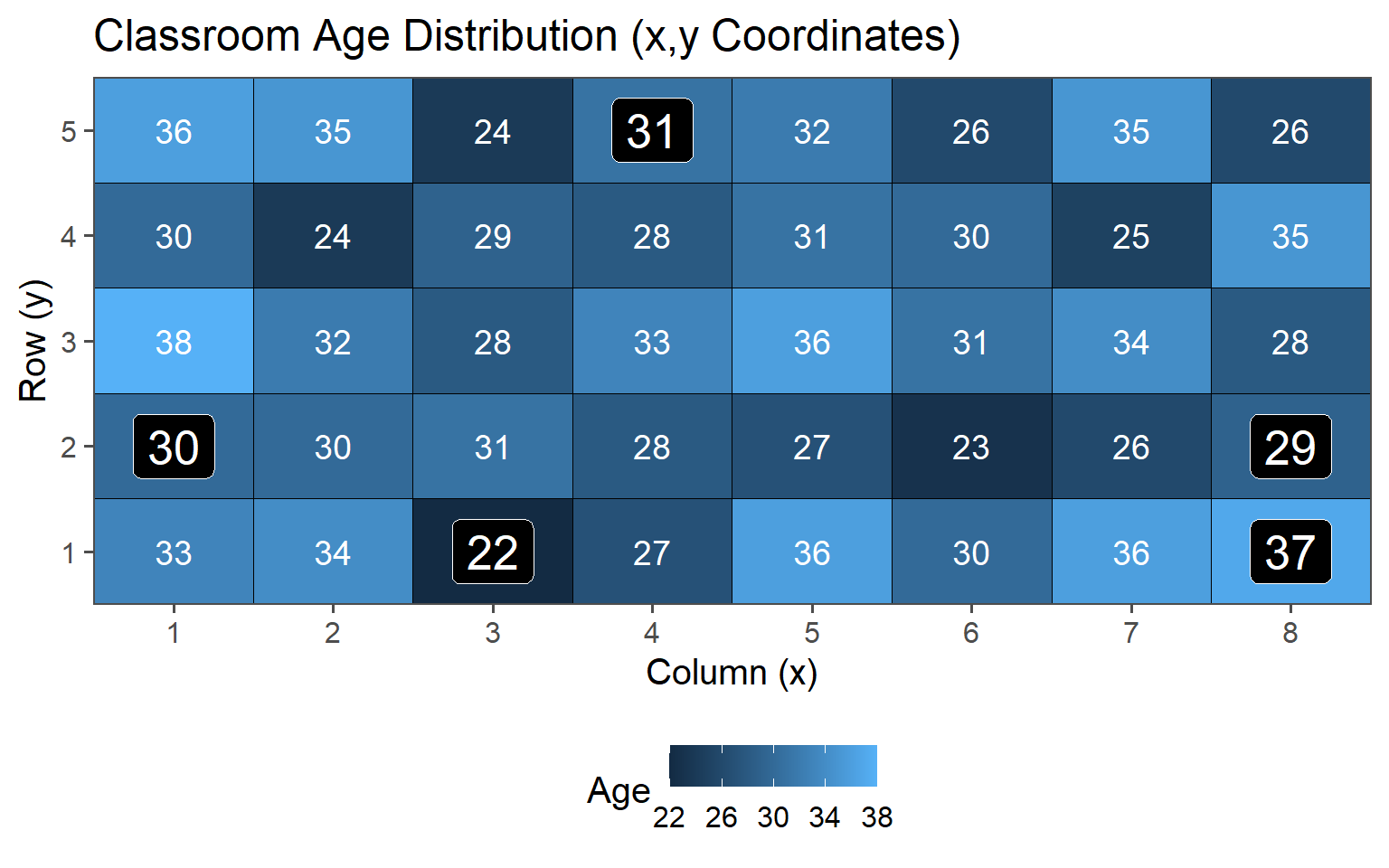
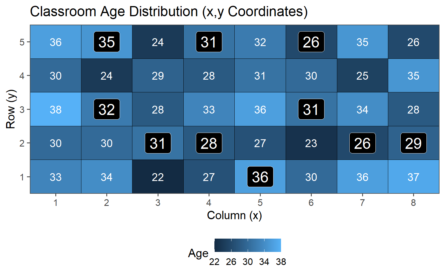
3.6.1.2 Classroom Age
3.6.1.3 Classroom Gender
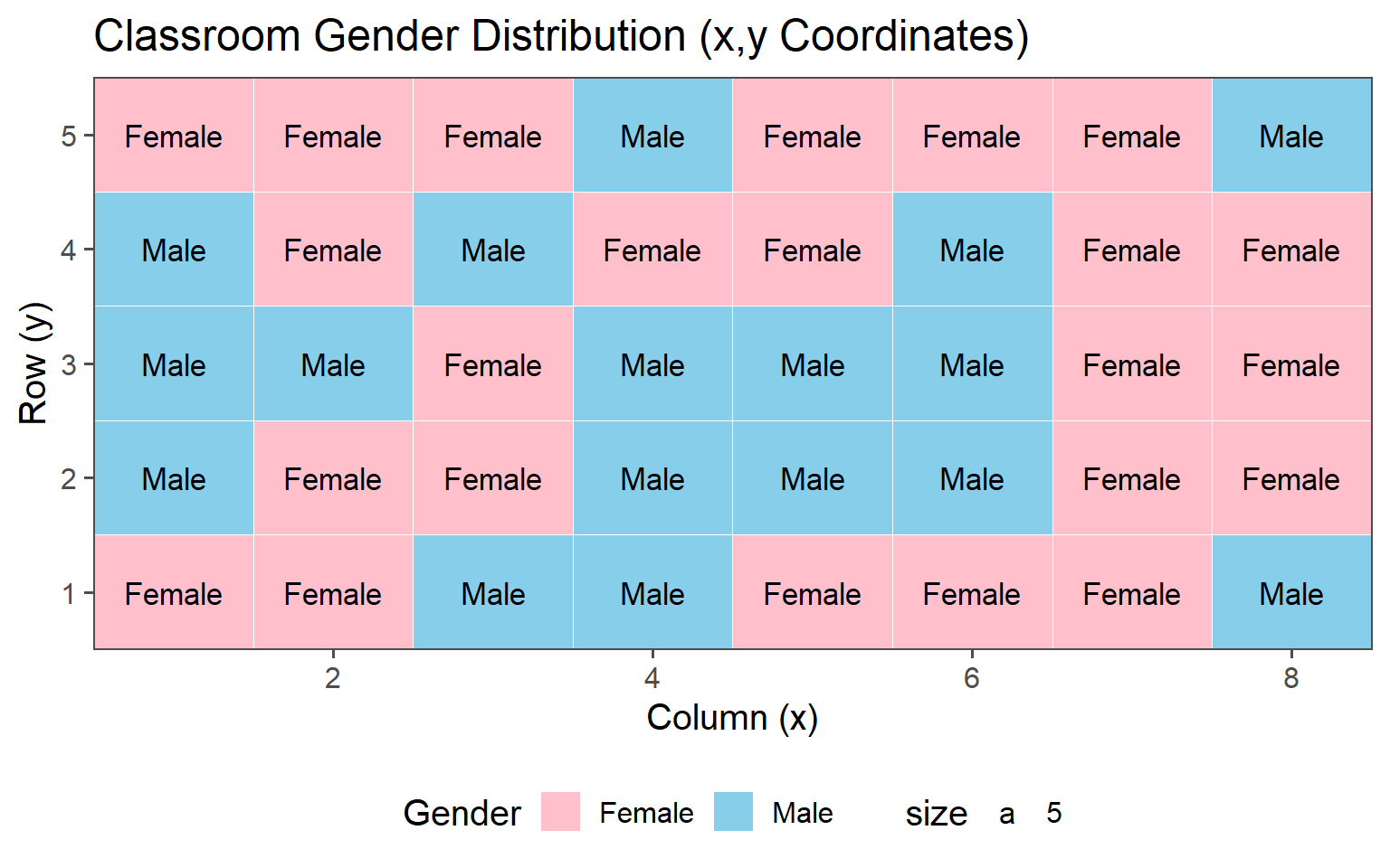
3.6.1.4 Population Values
\[\mu_{Age} = 30.4\] \[sd_{Age} = 4.18\]
These are the values we want to estimate using the introduced sampling strategies
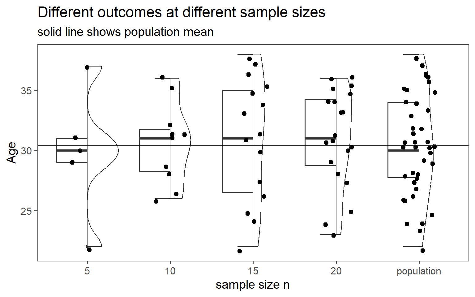
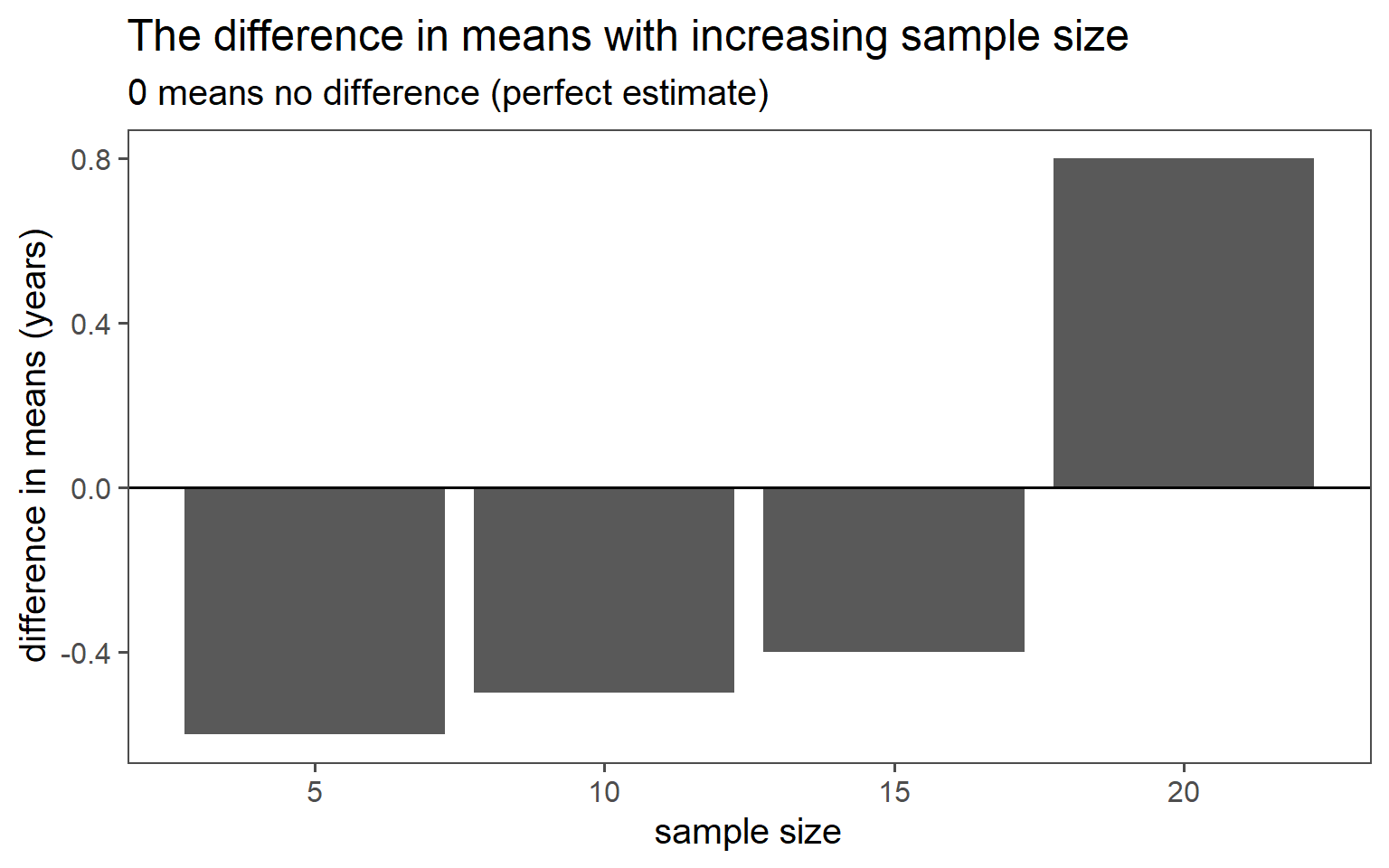
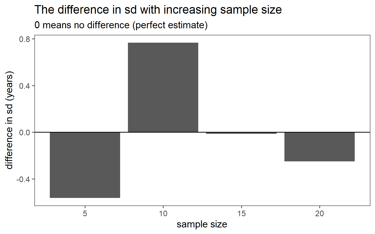
3.6.2 Simple Random Sampling
| n | mean in years | standard deviation in years |
|---|---|---|
| 5 | 29.80 | 5.36 |
| 10 | 30.50 | 3.37 |
| 15 | 30.93 | 5.09 |
| 20 | 31.00 | 4.00 |
| population | 30.40 | 4.18 |
3.6.2.1 \(n = 5\)
3.6.2.2 \(n = 10\)
3.6.2.3 \(n = 15\)
3.6.2.4 \(n = 20\)
3.6.2.5 Data
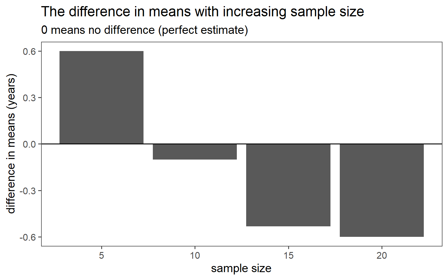
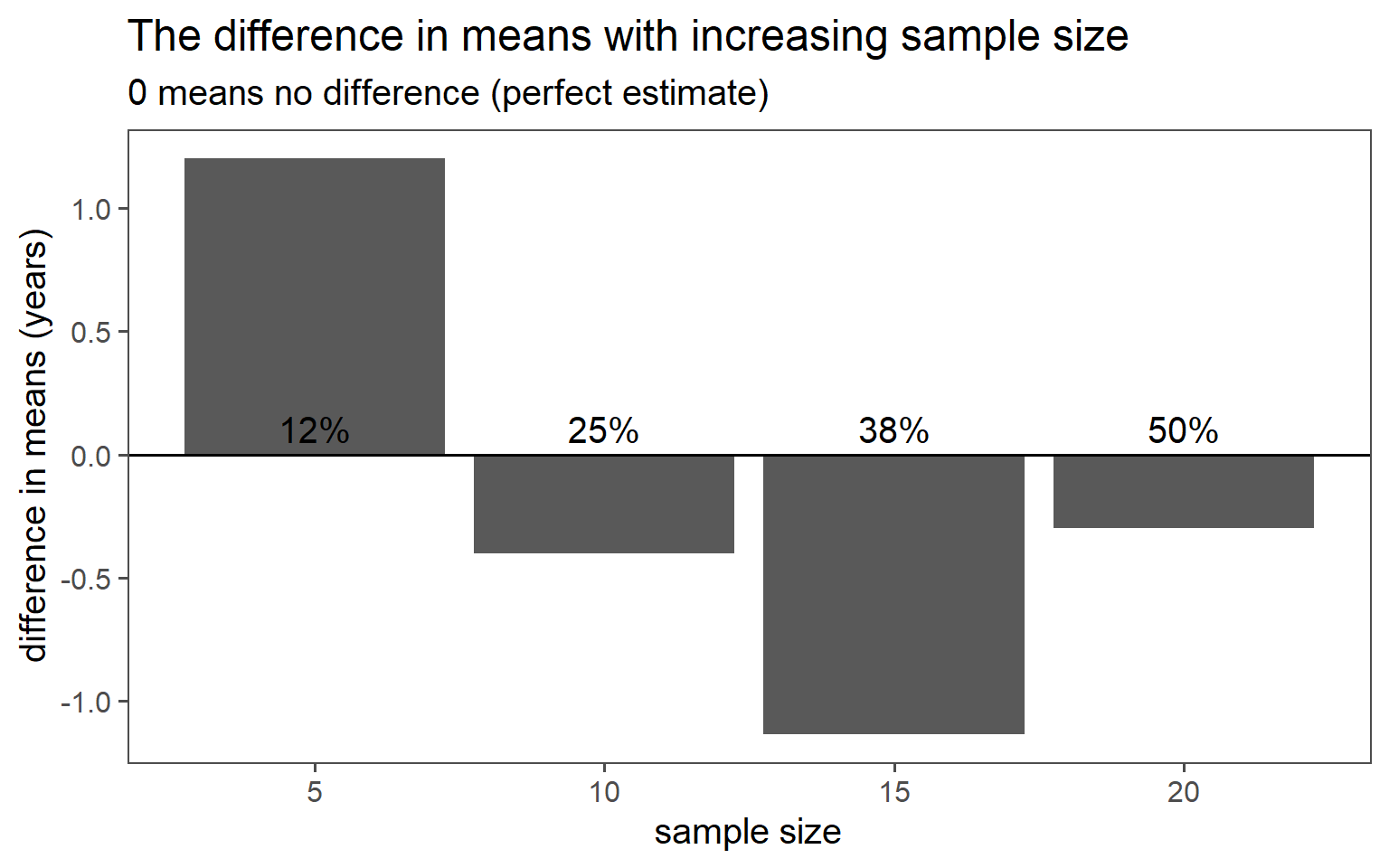
3.6.2.6 Mean Comparison
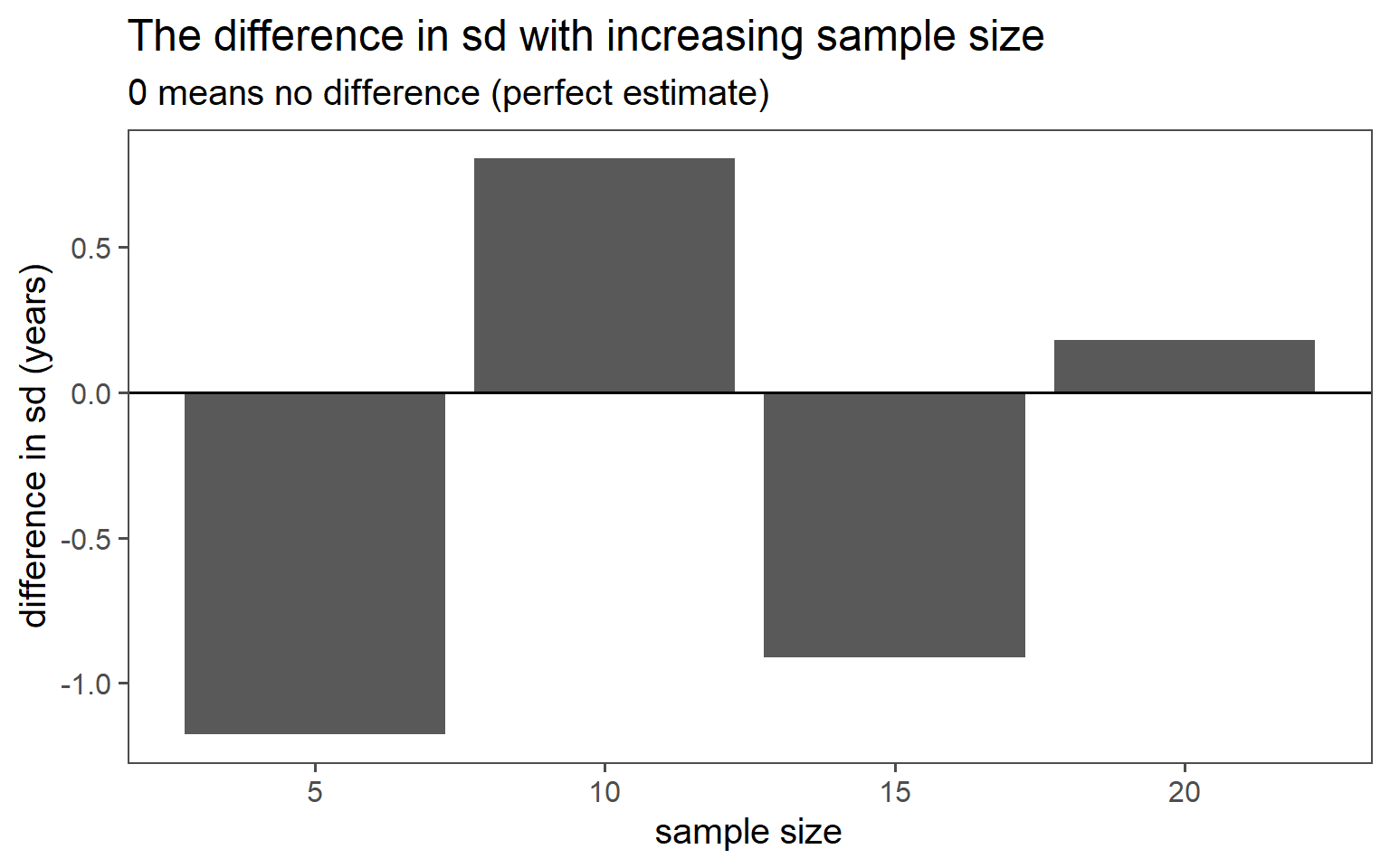
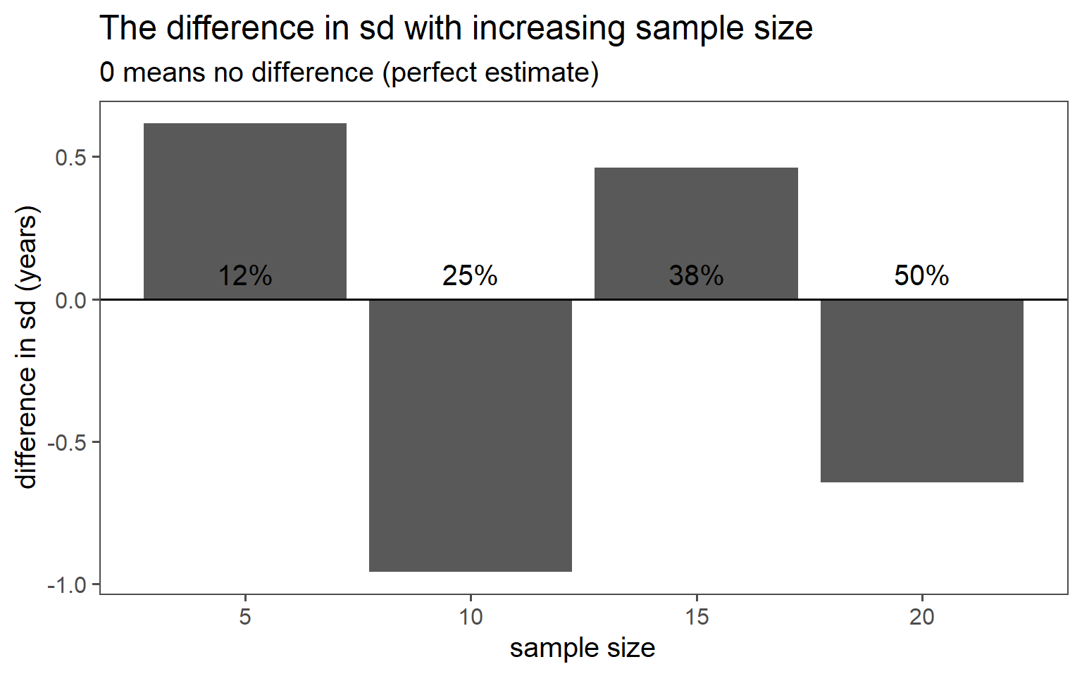
3.6.2.7 SD Comparison
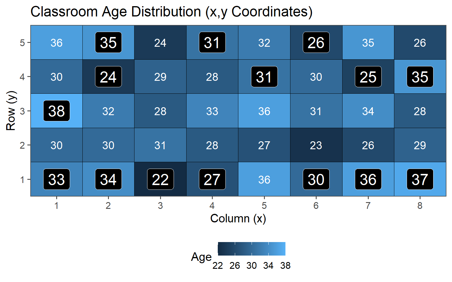
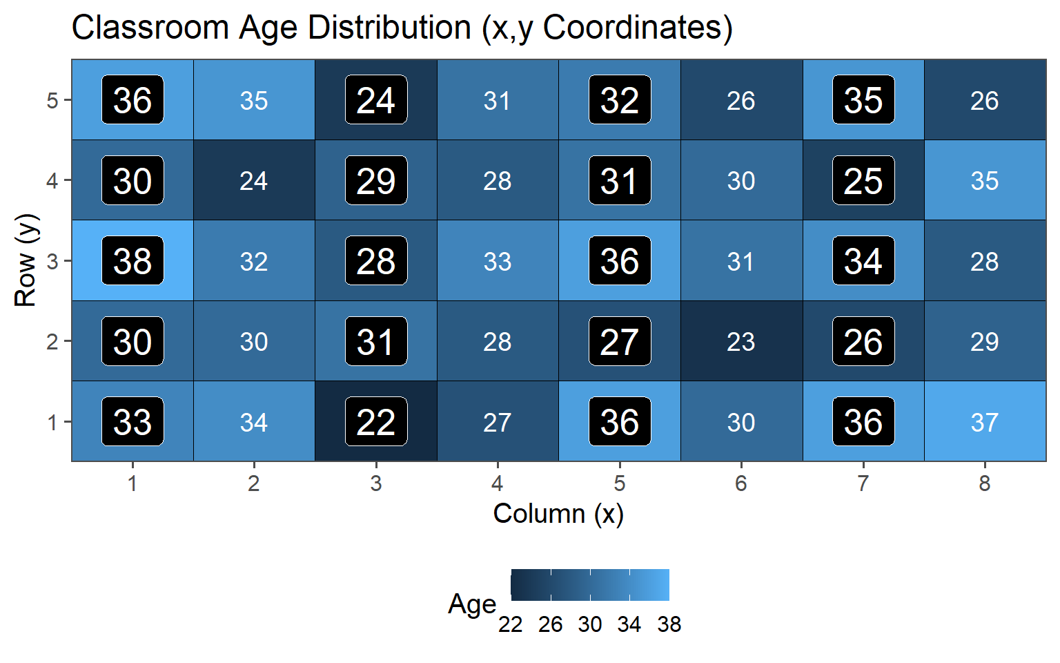
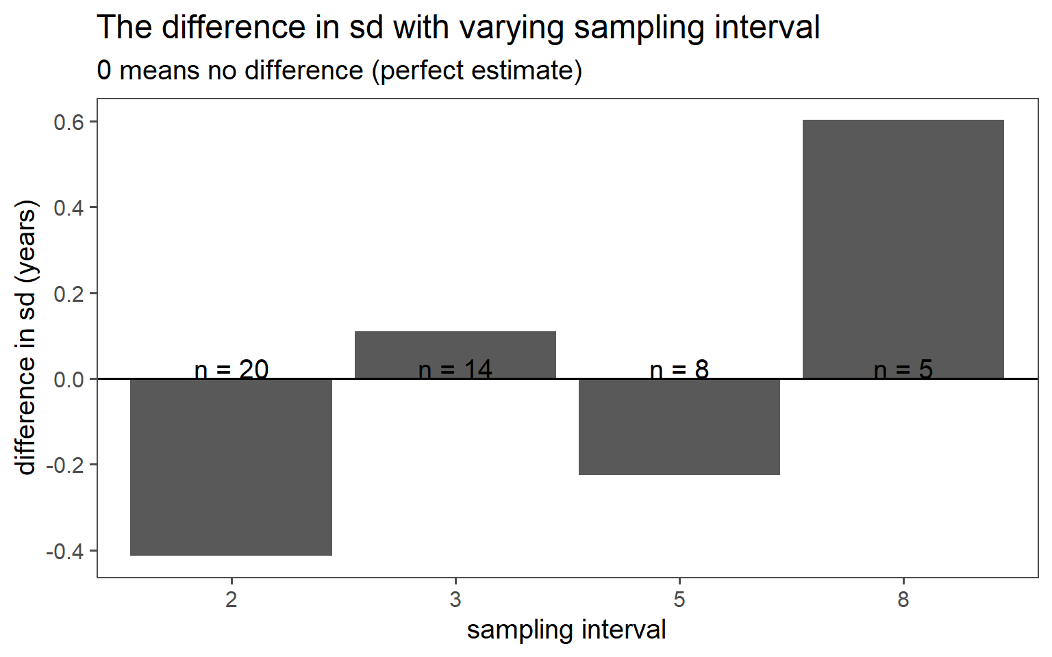
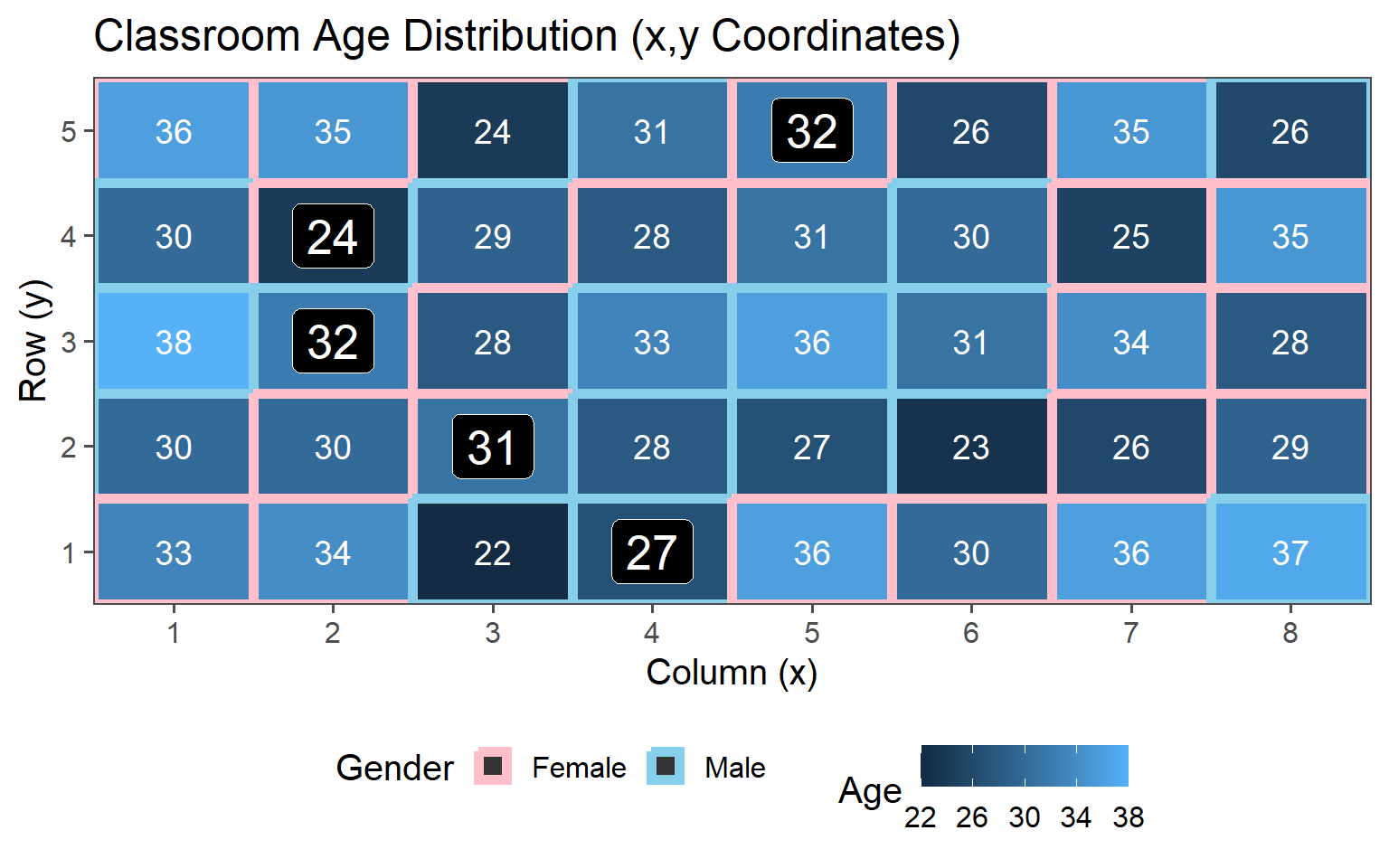
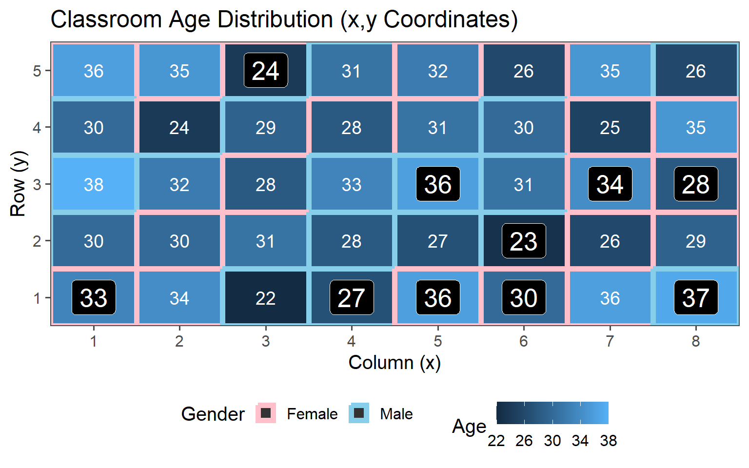
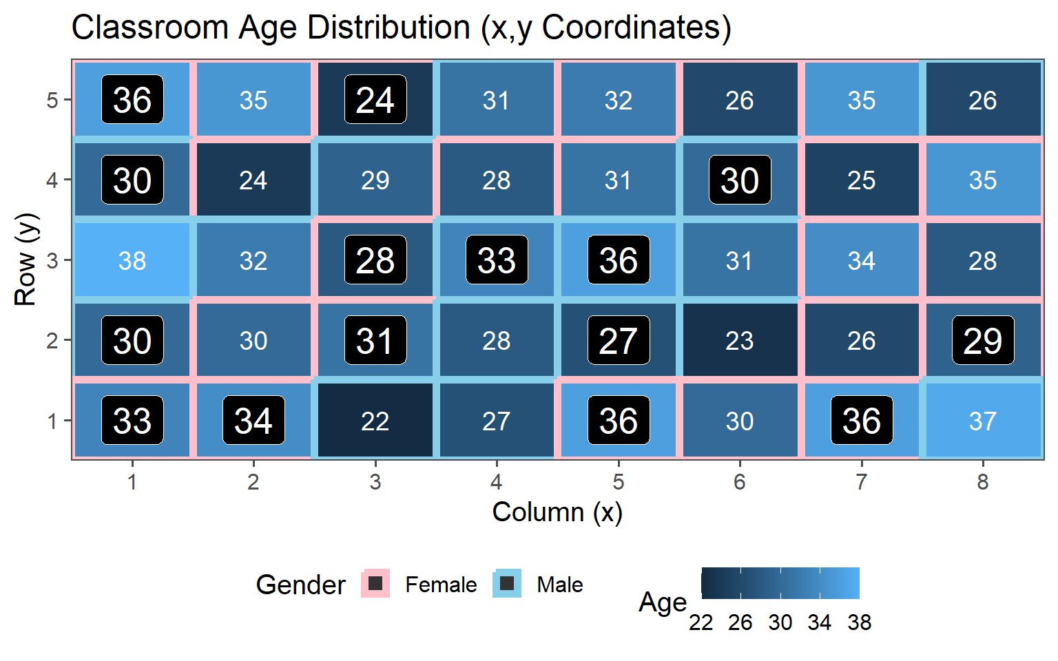
3.6.3 Systematic Sampling
Sample always the \(k\)th.
| k | mean in years | standard deviation in years |
|---|---|---|
| 8 | 33.40 | 3.58 |
| 5 | 30.62 | 4.41 |
| 3 | 31.57 | 4.07 |
| 2 | 30.95 | 4.59 |
| population | 30.40 | 4.18 |
3.6.3.1 \(k = 8\)
3.6.3.2 \(k = 5\)
3.6.3.3 \(k = 2\)
3.6.3.4 Data
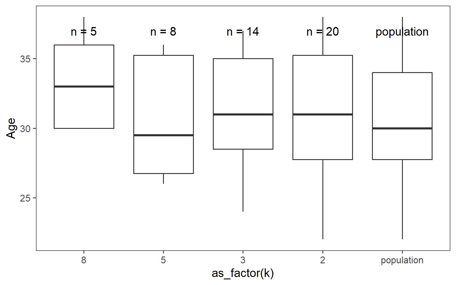
3.6.3.5 Mean Comparison

3.6.3.6 SD Comparison
3.6.4 Stratified Sampling
Choose sample stratified to characteristic (Gender represented in population)
3.6.4.1 \(\text{proportion} = 12\% \rightarrow n = 5\)
3.6.4.2 \(\text{proportion} = 25\% \rightarrow n = 10\)
3.6.4.3 \(\text{proportion} = 38\% \rightarrow n = 15\)
3.6.4.4 \(\text{proportion} = 50\% \rightarrow n = 20\)
3.6.4.5 Data

3.6.4.6 Mean Comparsion
3.6.4.7 SD Comparison
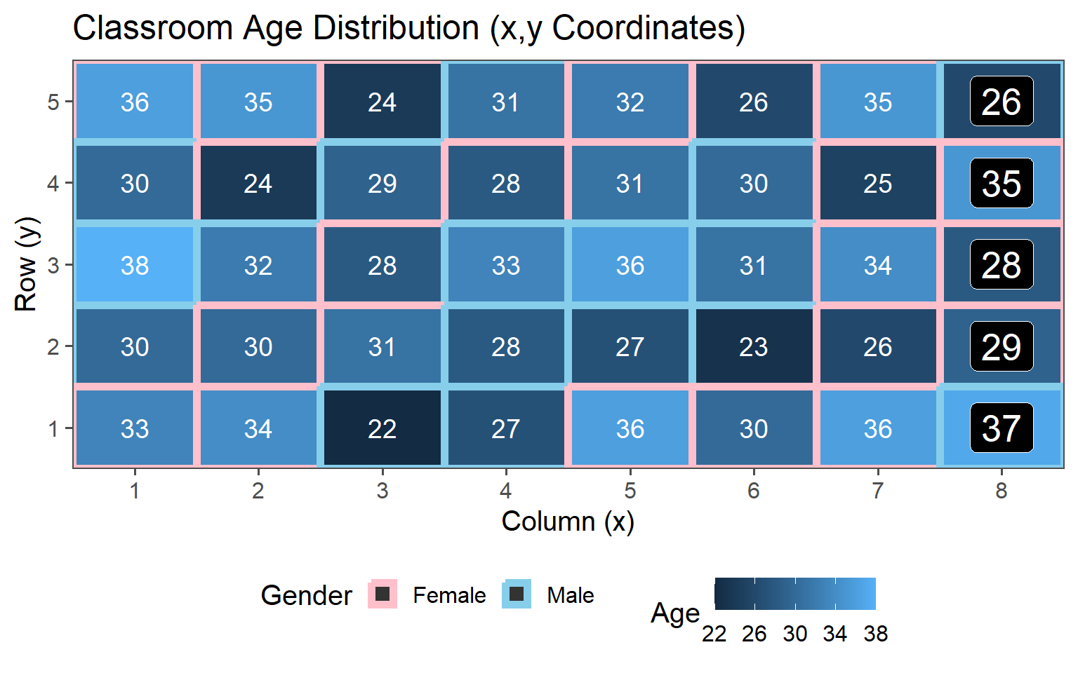
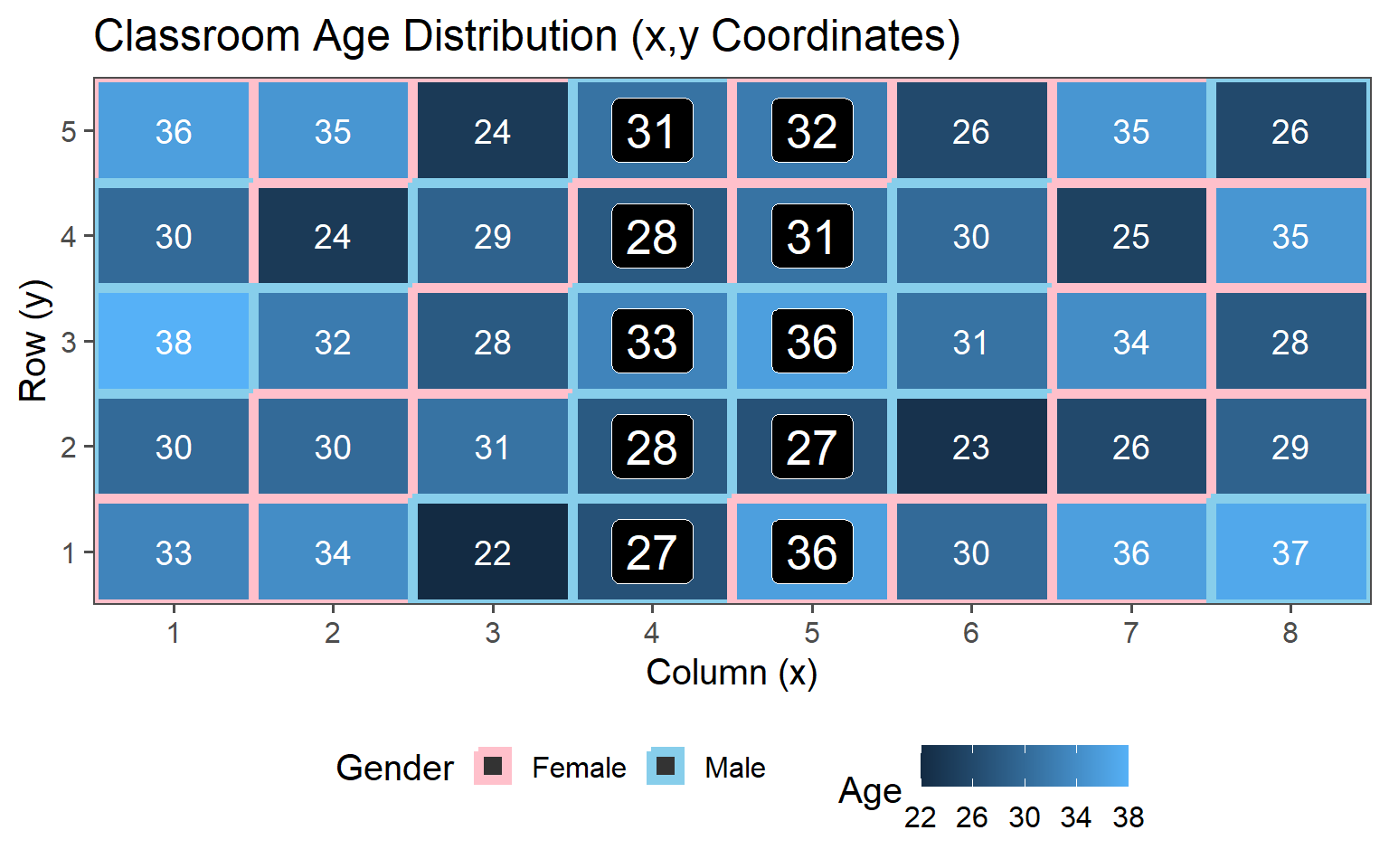
3.6.5 Clustered Sampling
Clusters are logical units which are sampled in order to save sampling resources.
In our case clusters are columns of students.
3.6.5.1 One Cluster
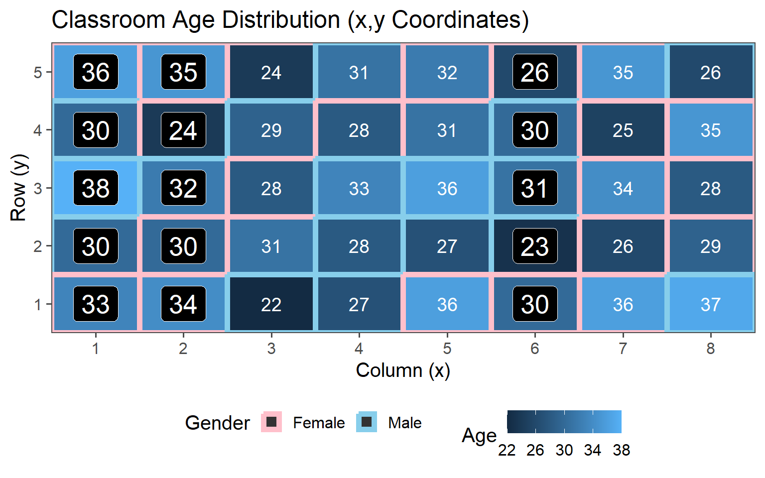
3.6.5.2 Two Clusters
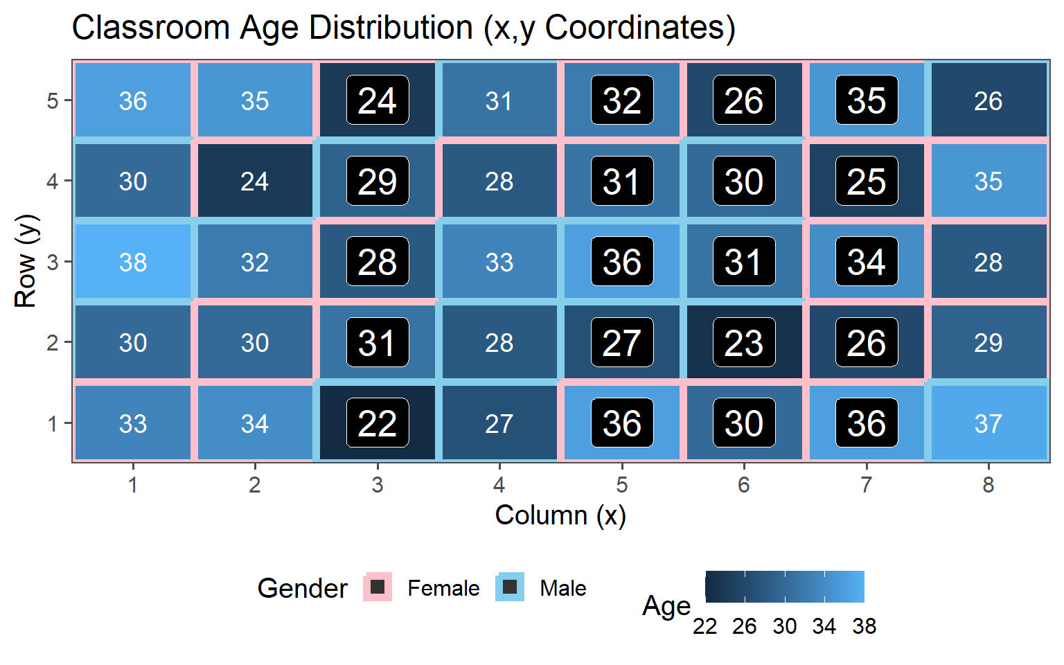
3.6.5.3 Three Clusters
3.6.5.4 Four Clusters
3.6.5.5 Data
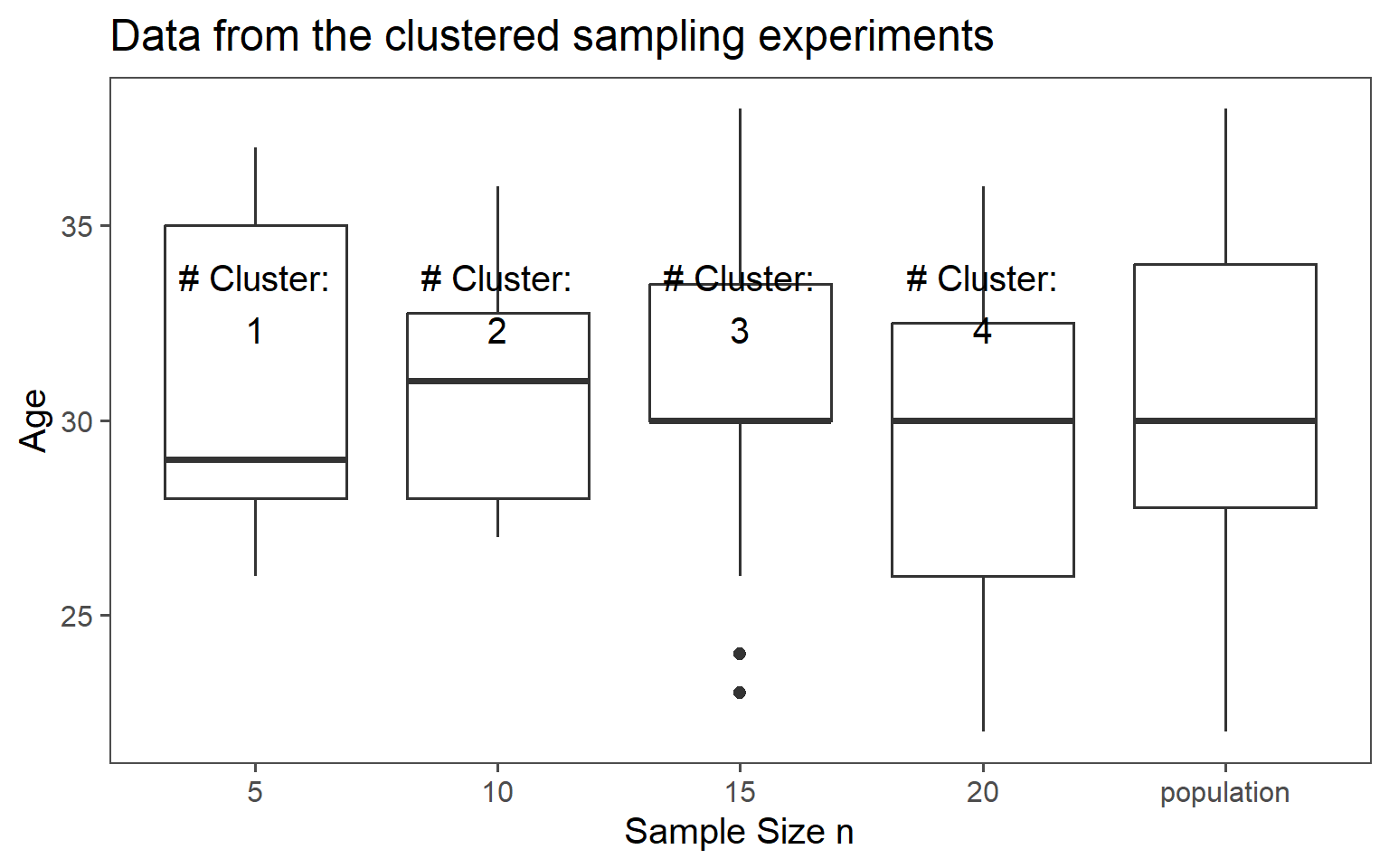
3.6.5.6 Mean Comparison
3.6.5.7 SD Comparison
3.6.6 Overall Comparison of Sampling Strategies (Gender)
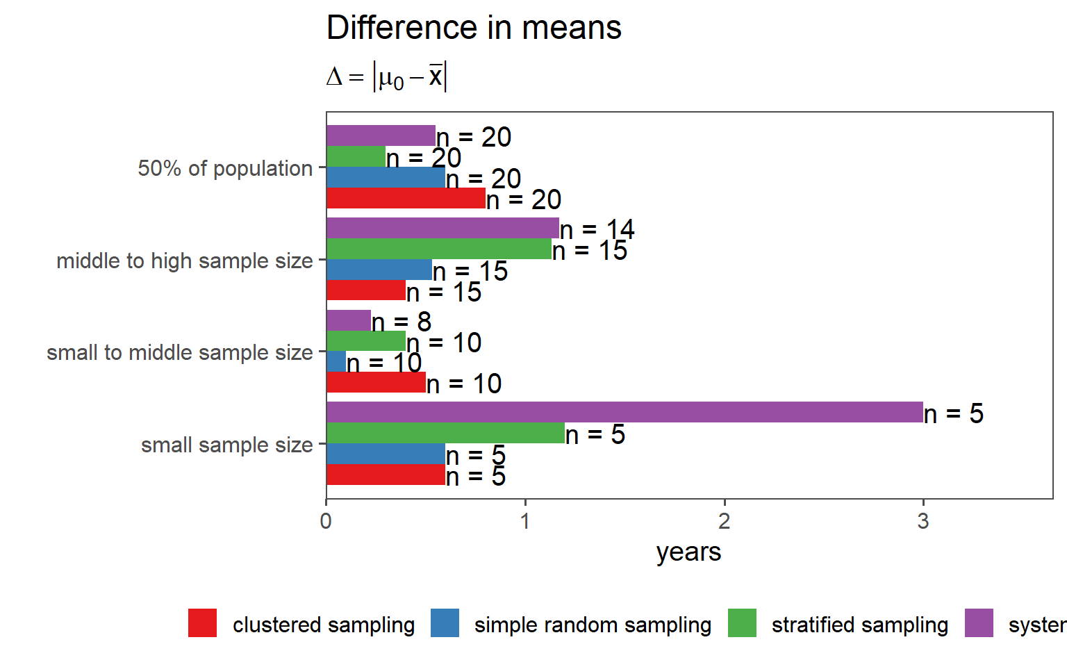
3.6.7 Overall Comparison of Sampling Strategies (Mean)
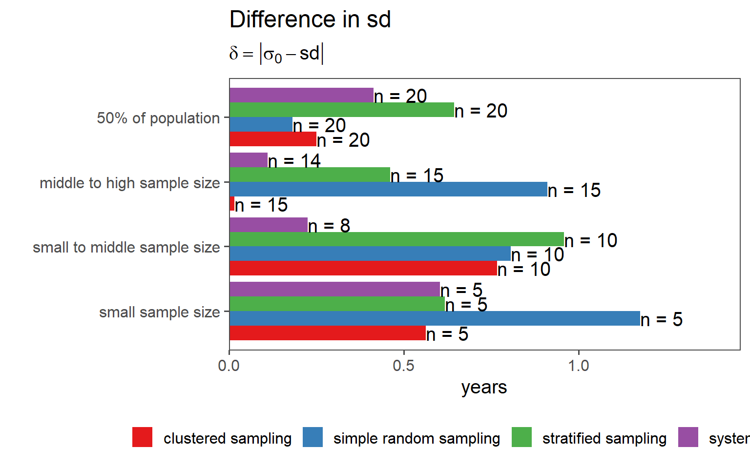
3.6.8 Overall Comparison of Sampling Strategies (SD)
3.7 Bootstrapping
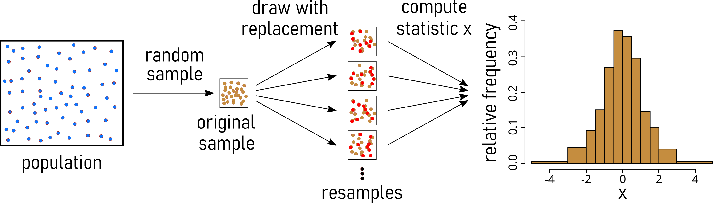
3.7.1 Bootstrapping in general
Definition: Estimating sample statistic distribution by drawing new samples with replacement from observed data, providing insights into variability without strict population distribution assumptions.
Advantages:
- Non-parametric: Works without assuming a specific data distribution.
- Confidence Intervals: Facilitates easy estimation of confidence intervals.
- Robustness: Reliable for small sample sizes or unknown data distributions.
Disadvantages:
- Computationally Intensive: Resource-intensive for large datasets.
- Results quality relies on the representativeness of the initial sample (garbage in - garbage out).
- Cannot compensate for inadequate information in the original sample.
- Not Always Optimal: Traditional methods may be better in cases meeting distribution assumptions.